重心插值器#
- class scipy.interpolate.BarycentricInterpolator(xi, yi=None, axis=0, *, wi=None, rng=None)[原始碼]#
一組點的插值多項式。
建構一個通過給定點集的 polynomial。 允許評估多項式及其所有導數,有效率地更改要插值的 y 值,以及透過新增更多 x 和 y 值來更新。
基於數值穩定性的考量,此函數不計算多項式的係數。
值 yi 需要在函數被評估之前提供,但沒有任何預處理依賴於它們,因此可以快速更新。
- 參數:
- xiarray_like,形狀 (npoints, )
多項式應通過的點的 x 坐標的 1-D 陣列
- yiarray_like,形狀 (…, npoints, …),可選
多項式應通過的點的 y 坐標的 N-D 陣列。 如果為 None,則 y 值將稍後通過 set_y 方法提供。沿插值軸的 yi 的長度必須等於 xi 的長度。 使用
axis參數選擇正確的軸。- axisint,可選
yi 陣列中對應於 x 坐標值的軸。 預設為
axis=0。- wiarray_like,可選
所選插值點 xi 的重心權重。 如果不存在或為 None,則權重將從 xi 計算 (預設)。 如果使用相同的節點 xi 計算多個插值器,則允許重複使用權重 wi,而無需重新計算。
- rng{None, int,
numpy.random.Generator}, 可選 如果通過關鍵字傳遞 rng,則除了
numpy.random.Generator之外的類型將傳遞給numpy.random.default_rng以實例化Generator。 如果 rng 已經是Generator實例,則使用提供的實例。 指定 rng 以進行可重複的插值。如果通過關鍵字傳遞此參數 random_state,則適用於參數 random_state 的舊版行為
如果 random_state 為 None (或
numpy.random),則使用numpy.random.RandomStatesingleton。如果 random_state 是一個整數,則使用新的
RandomState實例,並以 random_state 作為種子。如果 random_state 已經是
Generator或RandomState實例,則使用該實例。
在版本 1.15.0 中變更: 作為從使用
numpy.random.RandomState過渡到numpy.random.Generator的 SPEC-007 轉換的一部分,此關鍵字已從 random_state 變更為 rng。 在過渡期間,這兩個關鍵字將繼續工作 (僅指定其中一個)。 在過渡期之後,使用 random_state 關鍵字將發出警告。 random_state 和 rng 關鍵字的行為概述如上。
筆記
此類別使用“重心插值”方法,將問題視為有理函數插值的特例。 從數值上看,此演算法非常穩定,但即使在精確計算的世界中,除非非常仔細地選擇 x 坐標 - Chebyshev 零點 (例如,cos(i*pi/n)) 是一個不錯的選擇 - 否則由於 Runge 現象,多項式插值本身是一個病態過程。
基於 Berrut 和 Trefethen 2004,“重心拉格朗日插值”。
範例
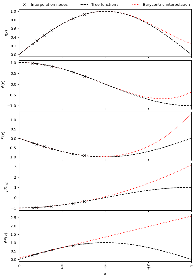
為了產生近似函數 \(\sin x\) 的五次重心插值器,及其前四個導數,使用 \((0, \frac{\pi}{2})\) 中六個隨機間隔的節點
>>> import numpy as np
>>> import matplotlib.pyplot as plt
>>> from scipy.interpolate import BarycentricInterpolator
>>> rng = np.random.default_rng()
>>> xi = rng.random(6) * np.pi/2
>>> f, f_d1, f_d2, f_d3, f_d4 = np.sin, np.cos, lambda x: -np.sin(x), lambda x: -np.cos(x), np.sin
>>> P = BarycentricInterpolator(xi, f(xi), random_state=rng)
>>> fig, axs = plt.subplots(5, 1, sharex=True, layout='constrained', figsize=(7,10))
>>> x = np.linspace(0, np.pi, 100)
>>> axs[0].plot(x, P(x), 'r:', x, f(x), 'k--', xi, f(xi), 'xk')
>>> axs[1].plot(x, P.derivative(x), 'r:', x, f_d1(x), 'k--', xi, f_d1(xi), 'xk')
>>> axs[2].plot(x, P.derivative(x, 2), 'r:', x, f_d2(x), 'k--', xi, f_d2(xi), 'xk')
>>> axs[3].plot(x, P.derivative(x, 3), 'r:', x, f_d3(x), 'k--', xi, f_d3(xi), 'xk')
>>> axs[4].plot(x, P.derivative(x, 4), 'r:', x, f_d4(x), 'k--', xi, f_d4(xi), 'xk')
>>> axs[0].set_xlim(0, np.pi)
>>> axs[4].set_xlabel(r"$x$")
>>> axs[4].set_xticks([i * np.pi / 4 for i in range(5)],
...                   ["0", r"$\frac{\pi}{4}$", r"$\frac{\pi}{2}$", r"$\frac{3\pi}{4}$", r"$\pi$"])
>>> axs[0].set_ylabel("$f(x)$")
>>> axs[1].set_ylabel("$f'(x)$")
>>> axs[2].set_ylabel("$f''(x)$")
>>> axs[3].set_ylabel("$f^{(3)}(x)$")
>>> axs[4].set_ylabel("$f^{(4)}(x)$")
>>> labels = ['Interpolation nodes', 'True function $f$', 'Barycentric interpolation']
>>> axs[0].legend(axs[0].get_lines()[::-1], labels, bbox_to_anchor=(0., 1.02, 1., .102),
...               loc='lower left', ncols=3, mode="expand", borderaxespad=0., frameon=False)
>>> plt.show()
- 屬性:
- dtype
方法
__call__(x)在點 x 評估插值多項式
add_xi(xi[, yi])將更多 x 值新增到要插值的集合
derivative(x[, der])在點 x 評估多項式的單個導數。
derivatives(x[, der])在點 x 評估多項式的多個導數
set_yi(yi[, axis])更新要插值的 y 值