scipy.signal.

czt#

scipy.signal.czt(x, m=None, w=None, a=1 + 0j, *, axis=-1)[source]#

計算 Z 平面螺旋周圍的頻率響應。

參數:

x陣列: 要轉換的訊號。
m整數，選用: 所需的輸出點數量。預設值為輸入資料的長度。
w複數，選用: 每步中點之間的比例。此值必須精確，否則累積誤差會降低輸出序列的尾部。預設為單位圓周圍均勻間隔的點。
a複數，選用: 複數平面中的起點。預設值為 1+0j。
axis整數，選用: 計算 FFT 的軸。如果未給定，則使用最後一個軸。

回傳值:

outndarray: 與 x 具有相同維度的陣列，但轉換軸的長度設定為 m。

另請參閱

CZT: 建立可呼叫的 chirp z 轉換函數的類別。
zoom_fft: 用於部分 FFT 計算的便利函數。

註解

預設值的選擇使得 signal.czt(x) 等同於 fft.fft(x)，並且，如果 m > len(x)，則 signal.czt(x, m) 等同於 fft.fft(x, m)。

如果需要重複轉換，請使用 CZT 來建構一個專用的轉換函數，該函數可以重複使用，而無需重新計算常數。

一個範例應用是在系統識別中，重複評估系統的 z 轉換的小切片，在預期存在極點的位置附近，以精確化極點真實位置的估計值。[1]

參考文獻

[1]

Steve Alan Shilling，“ chirp z 轉換及其應用研究”，第 20 頁 (1970) https://krex.k-state.edu/dspace/bitstream/handle/2097/7844/LD2668R41972S43.pdf

範例

產生一個正弦波

>>> import numpy as np
>>> f1, f2, fs = 8, 10, 200  # Hz
>>> t = np.linspace(0, 1, fs, endpoint=False)
>>> x = np.sin(2*np.pi*t*f2)
>>> import matplotlib.pyplot as plt
>>> plt.plot(t, x)
>>> plt.axis([0, 1, -1.1, 1.1])
>>> plt.show()

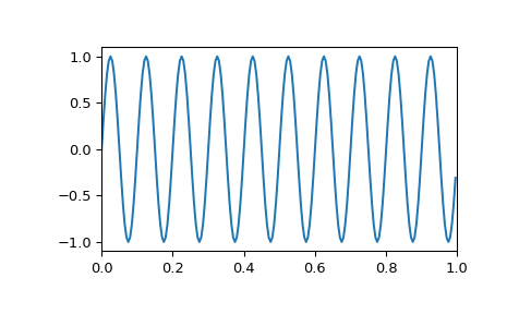
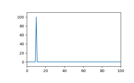
其離散傅立葉轉換的所有能量都集中在單個頻率 bin 中

>>> from scipy.fft import rfft, rfftfreq
>>> from scipy.signal import czt, czt_points
>>> plt.plot(rfftfreq(fs, 1/fs), abs(rfft(x)))
>>> plt.margins(0, 0.1)
>>> plt.show()

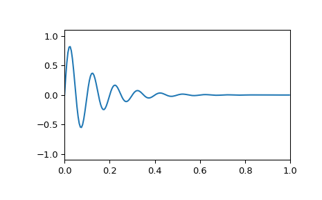
然而，如果正弦波是呈對數衰減的

>>> x = np.exp(-t*f1) * np.sin(2*np.pi*t*f2)
>>> plt.plot(t, x)
>>> plt.axis([0, 1, -1.1, 1.1])
>>> plt.show()

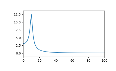
DFT 將會出現頻譜洩漏

>>> plt.plot(rfftfreq(fs, 1/fs), abs(rfft(x)))
>>> plt.margins(0, 0.1)
>>> plt.show()

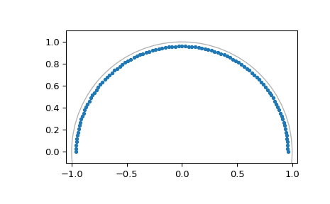
雖然 DFT 始終在單位圓周圍採樣 z 轉換，但 chirp z 轉換允許我們沿著任何對數螺旋採樣 Z 轉換，例如半徑小於 1 的圓

>>> M = fs // 2  # Just positive frequencies, like rfft
>>> a = np.exp(-f1/fs)  # Starting point of the circle, radius < 1
>>> w = np.exp(-1j*np.pi/M)  # "Step size" of circle
>>> points = czt_points(M + 1, w, a)  # M + 1 to include Nyquist
>>> plt.plot(points.real, points.imag, '.')
>>> plt.gca().add_patch(plt.Circle((0,0), radius=1, fill=False, alpha=.3))
>>> plt.axis('equal'); plt.axis([-1.05, 1.05, -0.05, 1.05])
>>> plt.show()

使用正確的半徑，這可以在沒有頻譜洩漏的情況下轉換衰減的正弦波（以及其他具有相同衰減率的波）

>>> z_vals = czt(x, M + 1, w, a)  # Include Nyquist for comparison to rfft
>>> freqs = np.angle(points)*fs/(2*np.pi)  # angle = omega, radius = sigma
>>> plt.plot(freqs, abs(z_vals))
>>> plt.margins(0, 0.1)
>>> plt.show()