Jarque-Bera 適合度檢定#
假設我們希望從量測值推斷醫學研究中成年男性人類的體重是否不呈常態分佈 [1]。體重 (磅) 記錄在下方的陣列 x 中。
import numpy as np
x = np.array([148, 154, 158, 160, 161, 162, 166, 170, 182, 195, 236])
Jarque-Bera 檢定 scipy.stats.jarque_bera 首先計算基於樣本偏度和峰度的統計量。
from scipy import stats
res = stats.jarque_bera(x)
res.statistic
6.982848237344646
由於常態分佈具有零偏度和零(「超額」或「Fisher」)峰度,因此對於從常態分佈中抽取的樣本,此統計量的值往往較低。
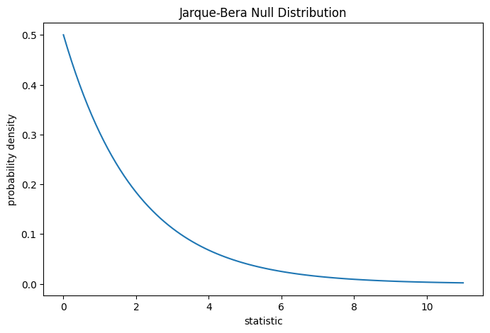
此檢定是透過將觀察到的統計量值與虛無分佈進行比較來執行的:虛無分佈是在體重是從常態分佈中抽取的虛無假設下得出的統計量值的分佈。
對於 Jarque-Bera 檢定,非常大樣本的虛無分佈是自由度為 2 的 卡方分佈。
import matplotlib.pyplot as plt

dist = stats.chi2(df=2)
jb_val = np.linspace(0, 11, 100)
pdf = dist.pdf(jb_val)
fig, ax = plt.subplots(figsize=(8, 5))

def jb_plot(ax):  # we'll reuse this
    ax.plot(jb_val, pdf)
    ax.set_title("Jarque-Bera Null Distribution")
    ax.set_xlabel("statistic")
    ax.set_ylabel("probability density")

jb_plot(ax)
plt.show();
比較結果以 p 值量化:虛無分佈中大於或等於觀察到的統計量值的比例。
fig, ax = plt.subplots(figsize=(8, 5))
jb_plot(ax)
pvalue = dist.sf(res.statistic)
annotation = (f'p-value={pvalue:.6f}\n(shaded area)')
props = dict(facecolor='black', width=1, headwidth=5, headlength=8)
_ = ax.annotate(annotation, (7.5, 0.01), (8, 0.05), arrowprops=props)
i = jb_val >= res.statistic  # indices of more extreme statistic values
ax.fill_between(jb_val[i], y1=0, y2=pdf[i])
ax.set_xlim(0, 11)
ax.set_ylim(0, 0.3)
plt.show()
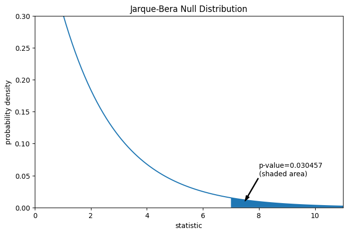
res.pvalue
0.03045746622458189
如果 p 值「很小」— 也就是說,如果從常態分佈族群中採樣資料產生如此極端統計量值的機率很低 — 這可以被視為反對虛無假設,而支持另一個假設的證據:體重不是從常態分佈中抽取的。請注意
反之則不然;也就是說,此檢定不用於提供支持虛無假設的證據。
將被視為「小」的值的閾值是一個應在分析資料之前做出的選擇 [2],並考量到偽陽性(錯誤地拒絕虛無假設)和偽陰性(未能拒絕錯誤的虛無假設)的風險。
請注意,卡方分佈提供了虛無分佈的漸近近似值;它僅適用於具有許多觀察值的樣本。對於像我們這樣的小樣本,scipy.stats.monte_carlo_test 可能提供更準確的、儘管是隨機的,精確 p 值的近似值。
def statistic(x, axis):
    # underlying calculation of the Jarque Bera statistic
    s = stats.skew(x, axis=axis)
    k = stats.kurtosis(x, axis=axis)
    return x.shape[axis]/6 * (s**2 + k**2/4)

res = stats.monte_carlo_test(x, stats.norm.rvs, statistic,
                             alternative='greater')
fig, ax = plt.subplots(figsize=(8, 5))
jb_plot(ax)
ax.hist(res.null_distribution, np.linspace(0, 10, 50),
        density=True)
ax.legend(['asymptotic approximation (many observations)',
           'Monte Carlo approximation (11 observations)'])
plt.show()
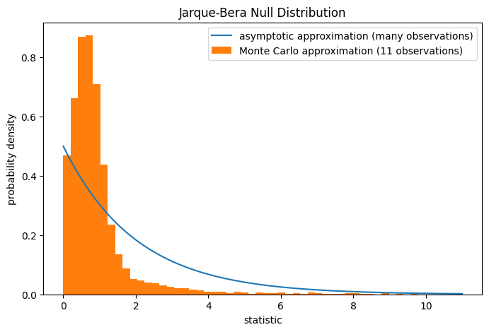
res.pvalue
0.0095
此外,儘管它們具有隨機性,但以這種方式計算的 p 值可用於精確控制虛無假設的錯誤拒絕率 [3]。