偏度檢定#
此函數檢定虛無假設,即樣本取自的母體的偏度與對應常態分佈的偏度相同。
假設我們希望從測量值推斷醫學研究中成年男性體重是否不呈常態分佈 [1]。體重 (磅) 記錄在下方的陣列 x 中。
import numpy as np
x = np.array([148, 154, 158, 160, 161, 162, 166, 170, 182, 195, 236])
偏度檢定 scipy.stats.skewtest 來自 [2],首先計算基於樣本偏度的統計量。
from scipy import stats
res = stats.skewtest(x)
res.statistic
2.7788579769903414
由於常態分佈的偏度為零,因此對於從常態分佈中抽取的樣本,此統計量的大小往往較小。
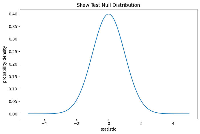
此檢定是透過將觀察到的統計量值與虛無分佈進行比較來執行的:虛無分佈是在虛無假設 (體重是從常態分佈中抽取的) 下導出的統計量值的分佈。
對於此檢定,極大樣本的統計量虛無分佈是標準常態分佈。
import matplotlib.pyplot as plt
dist = stats.norm()
st_val = np.linspace(-5, 5, 100)
pdf = dist.pdf(st_val)
fig, ax = plt.subplots(figsize=(8, 5))

def st_plot(ax):  # we'll reuse this
    ax.plot(st_val, pdf)
    ax.set_title("Skew Test Null Distribution")
    ax.set_xlabel("statistic")
    ax.set_ylabel("probability density")

st_plot(ax)
plt.show()
此比較以 p 值量化:虛無分佈中與觀察到的統計量值一樣極端或更極端的值的比例。在雙尾檢定中,虛無分佈中大於觀察到的統計量的值以及虛無分佈中小於觀察到的統計量的負數的值都被視為「更極端」。
fig, ax = plt.subplots(figsize=(8, 5))
st_plot(ax)
pvalue = dist.cdf(-res.statistic) + dist.sf(res.statistic)
annotation = (f'p-value={pvalue:.3f}\n(shaded area)')
props = dict(facecolor='black', width=1, headwidth=5, headlength=8)
_ = ax.annotate(annotation, (3, 0.005), (3.25, 0.02), arrowprops=props)
i = st_val >= res.statistic
ax.fill_between(st_val[i], y1=0, y2=pdf[i], color='C0')
i = st_val <= -res.statistic
ax.fill_between(st_val[i], y1=0, y2=pdf[i], color='C0')
ax.set_xlim(-5, 5)
ax.set_ylim(0, 0.1)
plt.show()
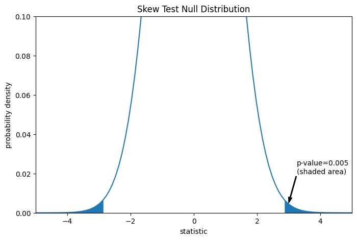
res.pvalue
0.005455036974740185
如果 p 值「很小」— 也就是說,如果從常態分佈母體中抽樣資料,產生如此極端的統計量值的機率很低 — 這可以被視為反對虛無假設,而支持對立假設的證據:體重並非從常態分佈中抽取。請注意,
反之則不然;也就是說,此檢定不用於提供支持虛無假設的證據。
將被視為「小」的值的閾值是一種選擇,應在分析資料之前做出 [3],並考慮偽陽性 (錯誤地拒絕虛無假設) 和偽陰性 (未能拒絕錯誤的虛無假設) 的風險。
請注意,標準常態分佈提供了虛無分佈的漸近近似值;它僅適用於具有大量觀察值的樣本。對於像我們這樣的小樣本,scipy.stats.monte_carlo_test 可能提供更準確,但具隨機性的精確 p 值近似值。
def statistic(x, axis):
    # get just the skewtest statistic; ignore the p-value
    return stats.skewtest(x, axis=axis).statistic

res = stats.monte_carlo_test(x, stats.norm.rvs, statistic)
fig, ax = plt.subplots(figsize=(8, 5))
st_plot(ax)
ax.hist(res.null_distribution, np.linspace(-5, 5, 50),
        density=True)
ax.legend(['asymptotic approximation\n(many observations)',
           'Monte Carlo approximation\n(11 observations)'])
plt.show()
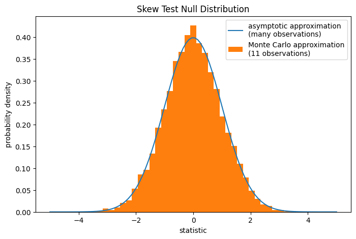
res.pvalue
0.0042
在本例中,即使對於我們的小樣本,漸近近似值和蒙地卡羅近似值也相當一致。