Spearman 相關係數#
Spearman 等級順序相關係數是一種用於衡量兩個資料集之間關係的單調性的非參數方法。
考慮以下來自 [1] 的資料,該研究探討了不健康人體肝臟中游離脯胺酸(一種胺基酸)和總膠原蛋白(一種常見於結締組織中的蛋白質)之間的關係。
下面的 x 和 y 陣列記錄了這兩種化合物的測量值。這些觀察值是成對的:每個游離脯胺酸測量值都取自與相同索引處的總膠原蛋白測量值相同的肝臟。
import numpy as np
# total collagen (mg/g dry weight of liver)
x = np.array([7.1, 7.1, 7.2, 8.3, 9.4, 10.5, 11.4])
# free proline (μ mole/g dry weight of liver)
y = np.array([2.8, 2.9, 2.8, 2.6, 3.5, 4.6, 5.0])
這些資料在 [2] 中使用 Spearman 相關係數進行了分析,這是一種對樣本之間單調相關性敏感的統計量,實作於 scipy.stats.spearmanr。
from scipy import stats
res = stats.spearmanr(x, y)
res.statistic
0.7000000000000001
對於具有強烈正序數相關的樣本,此統計量的值往往較高(接近 1);對於具有強烈負序數相關的樣本,此統計量的值往往較低(接近 -1);對於序數相關性較弱的樣本,此統計量的值在量級上較小(接近零)。
此檢定是透過將觀察到的統計量值與虛無分配進行比較來執行的:虛無分配是在總膠原蛋白和游離脯胺酸測量值獨立的虛無假設下得出的統計量值分配。
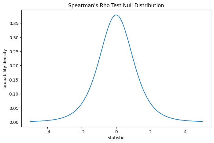
對於此檢定,可以轉換統計量,使得大樣本的虛無分配為自由度為 len(x) - 2 的 Student's t 分配。
import matplotlib.pyplot as plt
dof = len(x)-2  # len(x) == len(y)
dist = stats.t(df=dof)
t_vals = np.linspace(-5, 5, 100)
pdf = dist.pdf(t_vals)
fig, ax = plt.subplots(figsize=(8, 5))

def plot(ax):  # we'll reuse this
    ax.plot(t_vals, pdf)
    ax.set_title("Spearman's Rho Test Null Distribution")
    ax.set_xlabel("statistic")
    ax.set_ylabel("probability density")

plot(ax)
plt.show()
比較結果以 p 值量化:p 值是虛無分配中與觀察到的統計量值一樣極端或更極端的值的比例。在雙尾檢定中,如果統計量為正值,則虛無分配中大於轉換後統計量的值和虛無分配中小於觀察到的統計量值的負數的值都被視為「更極端」。
fig, ax = plt.subplots(figsize=(8, 5))
plot(ax)
rs = res.statistic  # original statistic
transformed = rs * np.sqrt(dof / ((rs+1.0)*(1.0-rs)))
pvalue = dist.cdf(-transformed) + dist.sf(transformed)
annotation = (f'p-value={pvalue:.4f}\n(shaded area)')
props = dict(facecolor='black', width=1, headwidth=5, headlength=8)
_ = ax.annotate(annotation, (2.7, 0.025), (3, 0.03), arrowprops=props)
i = t_vals >= transformed
ax.fill_between(t_vals[i], y1=0, y2=pdf[i], color='C0')
i = t_vals <= -transformed
ax.fill_between(t_vals[i], y1=0, y2=pdf[i], color='C0')
ax.set_xlim(-5, 5)
ax.set_ylim(0, 0.1)
plt.show()
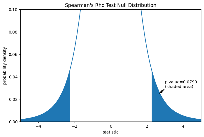
res.pvalue
0.07991669030889909
如果 p 值「很小」——也就是說,如果從獨立分配中採樣資料並產生如此極端的統計量值的機率很低——則這可以作為反對虛無假設而支持替代假設的證據:總膠原蛋白和游離脯胺酸的分配不是獨立的。請注意:
反之則不然;也就是說,該檢定不用於提供支持虛無假設的證據。
將被視為「小」的值的閾值是一個應在分析資料之前做出的選擇 [3],並考慮到偽陽性(錯誤地拒絕虛無假設)和偽陰性(未能拒絕錯誤的虛無假設)的風險。
小的 p 值並不是大效應的證據;相反,它們只能為「顯著」效應提供證據,這表示它們不太可能在虛無假設下發生。
假設在進行實驗之前,作者有理由預測總膠原蛋白和游離脯胺酸測量值之間存在正相關,並且他們選擇針對單尾替代方案評估虛無假設的合理性:游離脯胺酸與總膠原蛋白具有正序數相關性。在這種情況下,只有虛無分配中大於或等於觀察到的統計量的值才被認為是更極端的。
res = stats.spearmanr(x, y, alternative='greater')
res.statistic
0.7000000000000001
fig, ax = plt.subplots(figsize=(8, 5))
plot(ax)
pvalue = dist.sf(transformed)
annotation = (f'p-value={pvalue:.6f}\n(shaded area)')
props = dict(facecolor='black', width=1, headwidth=5, headlength=8)
_ = ax.annotate(annotation, (3, 0.018), (3.5, 0.03), arrowprops=props)
i = t_vals >= transformed
ax.fill_between(t_vals[i], y1=0, y2=pdf[i], color='C0')
ax.set_xlim(1, 5)
ax.set_ylim(0, 0.1)
plt.show()
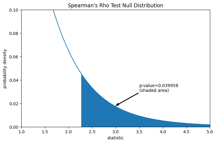
res.pvalue
0.03995834515444954
請注意,t 分配提供了虛無分配的漸近近似;它僅適用於具有大量觀察值的樣本。對於小樣本,執行置換檢定 [4] 可能更合適:在總膠原蛋白和游離脯胺酸獨立的虛無假設下,每個游離脯胺酸測量值都同樣有可能與任何總膠原蛋白測量值一起觀察到。因此,我們可以透過計算 x 和 y 之間元素每種可能的配對下的統計量來形成精確的虛無分配。
def statistic(x):  # explore all possible pairings by permuting `x`
    rs = stats.spearmanr(x, y).statistic  # ignore pvalue
    transformed = rs * np.sqrt(dof / ((rs+1.0)*(1.0-rs)))
    return transformed
ref = stats.permutation_test((x,), statistic, alternative='greater',
                             permutation_type='pairings')
fig, ax = plt.subplots(figsize=(8, 5))
plot(ax)
ax.hist(ref.null_distribution, np.linspace(-5, 5, 26),
        density=True)
ax.legend(['asymptotic approximation\n(many observations)',
           f'exact \n({len(ref.null_distribution)} permutations)'])
plt.show()
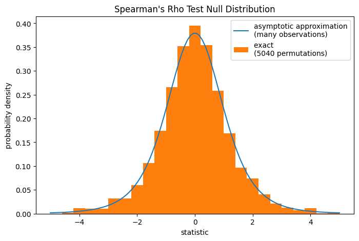
ref.pvalue
0.04563492063492063