Shapiro-Wilk 常態性檢定#
假設我們希望從量測值推斷一項醫學研究中成年男性人類的體重是否不呈常態分佈 [1]。體重(磅)記錄在下方的陣列 x 中。
import numpy as np
x = np.array([148, 154, 158, 160, 161, 162, 166, 170, 182, 195, 236])
常態性檢定 scipy.stats.shapiro 根據 [1] 和 [2] 開始計算一個統計量,該統計量基於觀測值與常態分佈的預期順序統計量之間的關係。
from scipy import stats
res = stats.shapiro(x)
res.statistic
0.7888146948631716
對於從常態分佈中抽取的樣本,此統計量的值往往會很高(接近 1)。
此檢定是透過將觀測到的統計量值與虛無分佈進行比較來執行的:虛無分佈是在體重是從常態分佈中抽取的虛無假設下形成的統計量值分佈。對於此常態性檢定,虛無分佈不容易精確計算,因此通常透過蒙地卡羅方法來近似,也就是從常態分佈中抽取許多與 x 相同大小的樣本,並計算每個樣本的統計量值。
def statistic(x):
# Get only the `shapiro` statistic; ignore its p-value
return stats.shapiro(x).statistic
ref = stats.monte_carlo_test(x, stats.norm.rvs, statistic,
alternative='less')
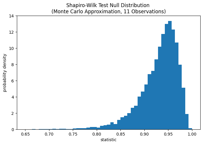
import matplotlib.pyplot as plt
fig, ax = plt.subplots(figsize=(8, 5))
bins = np.linspace(0.65, 1, 50)
def plot(ax): # we'll reuse this
ax.hist(ref.null_distribution, density=True, bins=bins)
ax.set_title("Shapiro-Wilk Test Null Distribution \n"
"(Monte Carlo Approximation, 11 Observations)")
ax.set_xlabel("statistic")
ax.set_ylabel("probability density")
plot(ax)
plt.show()
比較結果以 p 值量化:p 值是虛無分佈中小於或等於觀測到的統計量值的比例。
fig, ax = plt.subplots(figsize=(8, 5))
plot(ax)
annotation = (f'p-value={res.pvalue:.6f}\n(highlighted area)')
props = dict(facecolor='black', width=1, headwidth=5, headlength=8)
_ = ax.annotate(annotation, (0.75, 0.1), (0.68, 0.7), arrowprops=props)
i_extreme = np.where(bins <= res.statistic)[0]
for i in i_extreme:
    ax.patches[i].set_color('C1')
plt.xlim(0.65, 0.9)
plt.ylim(0, 4)
plt.show()
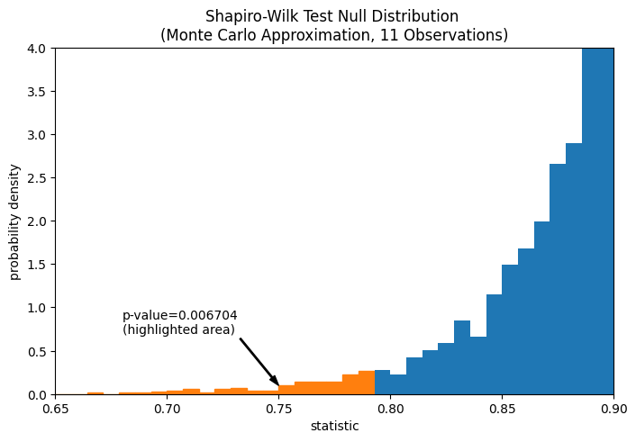
res.pvalue
0.006703814061898823
如果 p 值「很小」——也就是說,如果從常態分佈母體中抽樣資料並產生如此極端的統計量值的機率很低——這可以被視為反對虛無假設而支持另一種假設的證據:體重不是從常態分佈中抽取的。請注意
反之則不然;也就是說,此檢定不用於提供支持虛無假設的證據。
將被視為「小」的值的閾值是一個應該在分析資料之前做出的選擇 [3],並考慮到偽陽性(錯誤地拒絕虛無假設)和偽陰性(未能拒絕錯誤的虛無假設)的風險。