常態檢定#
scipy.stats.normaltest 函數檢定樣本是否來自常態分佈的虛無假設。它基於 D’Agostino 和 Pearson 的 [1] [2] 檢定,該檢定結合了偏度和峰度,以產生常態性的綜合檢定。
假設我們希望從測量值推斷醫學研究中成年男性體重是否不是常態分佈 [3]。體重(磅)記錄在下面的陣列 x 中。
import numpy as np
x = np.array([148, 154, 158, 160, 161, 162, 166, 170, 182, 195, 236])
常態性檢定 scipy.stats.normaltest 基於 [1] 和 [2],首先計算基於樣本偏度和峰度的統計量。
from scipy import stats
res = stats.normaltest(x)
res.statistic
/home/treddy/github_projects/scipy/doc/build/env/lib/python3.10/site-packages/scipy/stats/_axis_nan_policy.py:430: UserWarning: `kurtosistest` p-value may be inaccurate with fewer than 20 observations; only n=11 observations were given.
  return hypotest_fun_in(*args, **kwds)
13.034263121192582
(該檢定警告我們的樣本觀察值太少,無法執行檢定。我們將在本範例的結尾再回到這一點。)由於常態分佈具有零偏度和零(「超額」或「費雪」)峰度,因此對於從常態分佈中抽取的樣本,此統計量的值往往較低。
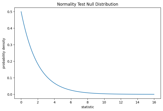
該檢定是通過將觀察到的統計量值與虛無分佈進行比較來執行的:虛無分佈是在體重是從常態分佈中抽取的虛無假設下得出的統計量值的分佈。對於此常態性檢定,極大樣本的虛無分佈是自由度為 2 的卡方分佈。
import matplotlib.pyplot as plt
dist = stats.chi2(df=2)
stat_vals = np.linspace(0, 16, 100)
pdf = dist.pdf(stat_vals)
fig, ax = plt.subplots(figsize=(8, 5))

def plot(ax):  # we'll reuse this
    ax.plot(stat_vals, pdf)
    ax.set_title("Normality Test Null Distribution")
    ax.set_xlabel("statistic")
    ax.set_ylabel("probability density")

plot(ax)
plt.show()
比較結果以 p 值量化:虛無分佈中大於或等於觀察到的統計量值的比例。
fig, ax = plt.subplots(figsize=(8, 5))
plot(ax)
pvalue = dist.sf(res.statistic)
annotation = (f'p-value={pvalue:.6f}\n(shaded area)')
props = dict(facecolor='black', width=1, headwidth=5, headlength=8)
_ = ax.annotate(annotation, (13.5, 5e-4), (14, 5e-3), arrowprops=props)
i = stat_vals >= res.statistic  # index more extreme statistic values
ax.fill_between(stat_vals[i], y1=0, y2=pdf[i])
ax.set_xlim(8, 16)
ax.set_ylim(0, 0.01)
plt.show()
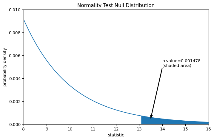
res.pvalue
0.0014779023013100172
如果 p 值「很小」——也就是說,如果從常態分佈族群中抽樣數據以產生如此極端的統計量值的機率很低——這可以被視為反對虛無假設而支持備擇假設的證據:體重不是從常態分佈中抽取的。請注意
反之則不然;也就是說,該檢定不用於為虛無假設提供證據。
將被視為「小」的值的閾值是一種選擇,應在分析數據之前做出 [4],並考慮假陽性(錯誤地拒絕虛無假設)和假陰性(未能拒絕錯誤的虛無假設)的風險。
請注意,卡方分佈提供了虛無分佈的漸近近似;它僅對具有許多觀察值的樣本準確。這就是我們在本範例開始時收到警告的原因;我們的樣本非常小。在這種情況下,scipy.stats.monte_carlo_test 可能提供更準確的,儘管是隨機的,精確 p 值的近似值。
def statistic(x, axis):
    # Get only the `normaltest` statistic; ignore approximate p-value
    return stats.normaltest(x, axis=axis).statistic
res = stats.monte_carlo_test(x, stats.norm.rvs, statistic,
                             alternative='greater')
fig, ax = plt.subplots(figsize=(8, 5))
plot(ax)
ax.hist(res.null_distribution, np.linspace(0, 25, 50),
        density=True)
ax.legend(['asymptotic approximation (many observations)',
           'Monte Carlo approximation (11 observations)'])
ax.set_xlim(0, 14)
plt.show()
/home/treddy/github_projects/scipy/doc/build/env/lib/python3.10/site-packages/scipy/stats/_axis_nan_policy.py:430: UserWarning: `kurtosistest` p-value may be inaccurate with fewer than 20 observations; only n=11 observations were given.
  return hypotest_fun_in(*args, **kwds)
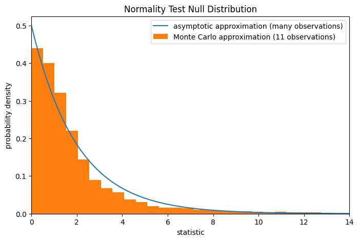
res.pvalue
0.0085
此外,儘管它們具有隨機性,但以這種方式計算的 p 值可用於精確控制虛無假設的錯誤拒絕率 [5]。