Levene 檢定變異數同質性#
Levene 檢定 scipy.stats.levene 檢定所有輸入樣本是否來自具有相同變異數的母體的虛無假設。在顯著偏離常態分佈的情況下,Levene 檢定是 Bartlett 檢定 scipy.stats.bartlett 的替代方案。
在 [1] 中,研究了維生素 C 對天竺鼠牙齒生長的影響。在一項對照研究中,60 名受試者被分為小劑量、中劑量和大劑量組,分別每天接受 0.5、1.0 和 2.0 毫克維生素 C 的劑量。42 天後,測量了牙齒生長情況。
下面的 small_dose、medium_dose 和 large_dose 陣列記錄了三組的牙齒生長測量值,單位為微米。
import numpy as np
small_dose = np.array([
    4.2, 11.5, 7.3, 5.8, 6.4, 10, 11.2, 11.2, 5.2, 7,
    15.2, 21.5, 17.6, 9.7, 14.5, 10, 8.2, 9.4, 16.5, 9.7
])
medium_dose = np.array([
    16.5, 16.5, 15.2, 17.3, 22.5, 17.3, 13.6, 14.5, 18.8, 15.5,
    19.7, 23.3, 23.6, 26.4, 20, 25.2, 25.8, 21.2, 14.5, 27.3
])
large_dose = np.array([
    23.6, 18.5, 33.9, 25.5, 26.4, 32.5, 26.7, 21.5, 23.3, 29.5,
    25.5, 26.4, 22.4, 24.5, 24.8, 30.9, 26.4, 27.3, 29.4, 23
])
scipy.stats.levene 統計量對樣本之間變異數的差異很敏感。
from scipy import stats
res = stats.levene(small_dose, medium_dose, large_dose)
res.statistic
0.6457341109631506
當變異數存在很大差異時,統計量的值往往會很高。
我們可以通過將觀察到的統計量值與虛無分佈進行比較,來檢定組間變異數的不相等性:虛無分佈是在虛無假設(即三組的母體變異數相等)下得出的統計量值的分佈。
對於此檢定,虛無分佈遵循 F 分佈,如下所示。
import matplotlib.pyplot as plt
k, n = 3, 60   # number of samples, total number of observations
dist = stats.f(dfn=k-1, dfd=n-k)
val = np.linspace(0, 5, 100)
pdf = dist.pdf(val)
fig, ax = plt.subplots(figsize=(8, 5))

def plot(ax):  # we'll reuse this
    ax.plot(val, pdf, color='C0')
    ax.set_title("Levene Test Null Distribution")
    ax.set_xlabel("statistic")
    ax.set_ylabel("probability density")
    ax.set_xlim(0, 5)
    ax.set_ylim(0, 1)

plot(ax)
plt.show()
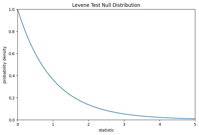
比較結果以 p 值量化:p 值是虛無分佈中大於或等於觀察到的統計量值的比例。
fig, ax = plt.subplots(figsize=(8, 5))
plot(ax)
pvalue = dist.sf(res.statistic)
annotation = (f'p-value={pvalue:.3f}\n(shaded area)')
props = dict(facecolor='black', width=1, headwidth=5, headlength=8)
_ = ax.annotate(annotation, (1.5, 0.22), (2.25, 0.3), arrowprops=props)
i = val >= res.statistic
ax.fill_between(val[i], y1=0, y2=pdf[i], color='C0')
plt.show()
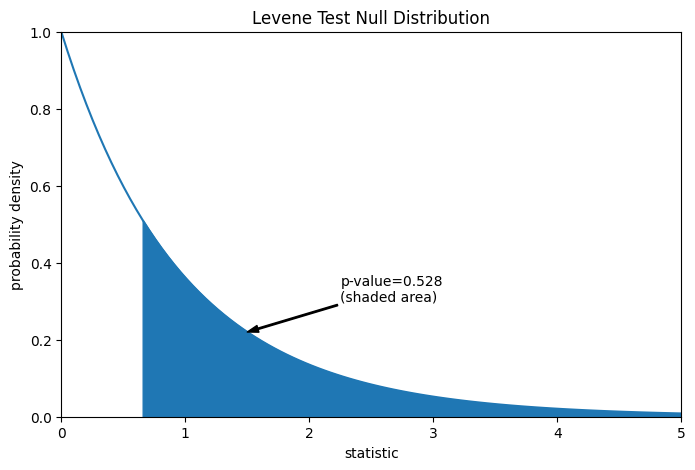
res.pvalue
0.5280694573759905
如果 p 值「很小」——也就是說,如果從具有相同變異數的分佈中抽樣數據,產生如此極端的統計量值的機率很低——這可以作為反對虛無假設,而支持對立假設的證據:各組的變異數不相等。請注意,
反之則不然;也就是說,該檢定不用於為虛無假設提供證據。
將被視為「小」的值的閾值是一個選擇,應在分析數據之前做出 [2],並考慮到假陽性(錯誤地拒絕虛無假設)和假陰性(未能拒絕錯誤的虛無假設)的風險。
小的 p 值並不是 large 效應的證據;相反,它們只能為「顯著」效應提供證據,這意味著它們不太可能在虛無假設下發生。
請注意,F 分佈提供了虛無分佈的漸近近似。對於小樣本,執行置換檢定可能更合適:在所有三個樣本都來自同一母體的虛無假設下,每個測量值都同樣有可能在三個樣本中的任何一個中被觀察到。因此,我們可以通過計算在許多隨機生成的將觀察值劃分到三個樣本中的情況下的統計量,來形成隨機化的虛無分佈。
def statistic(*samples):
    return stats.levene(*samples).statistic
ref = stats.permutation_test(
    (small_dose, medium_dose, large_dose), statistic,
    permutation_type='independent', alternative='greater'
)
fig, ax = plt.subplots(figsize=(8, 5))
plot(ax)
bins = np.linspace(0, 5, 25)
ax.hist(
    ref.null_distribution, bins=bins, density=True, facecolor="C1"
)
ax.legend(['asymptotic approximation\n(many observations)',
           'randomized null distribution'])
plot(ax)
plt.show()
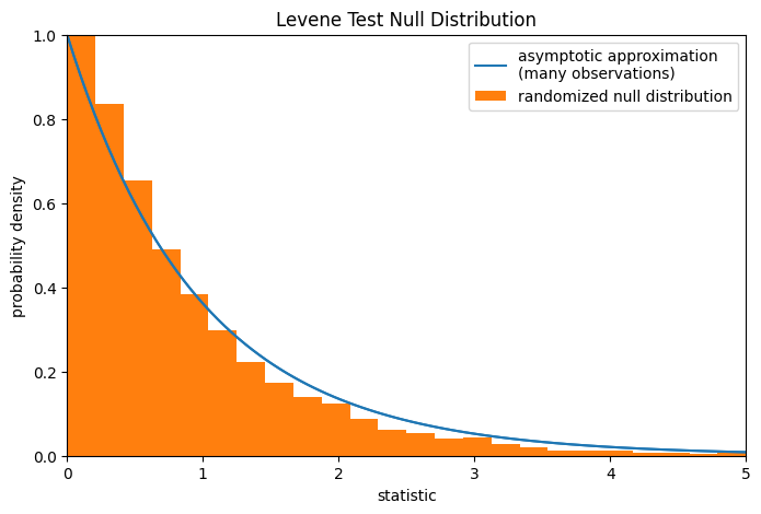
ref.pvalue # randomized test p-value
0.4565
請注意,此處計算的 p 值與 scipy.stats.levene 上面返回的漸近近似值之間存在顯著差異。可以從置換檢定中嚴格得出的統計推斷是有限的;儘管如此,在許多情況下,它們可能是首選方法 [3]。