scipy.signal.windows.

dpss

scipy.signal.windows.dpss(M, NW, Kmax=None, sym=True, norm=None, return_ratios=False)

計算離散長球面序列 (DPSS)。

DPSS（或 Slepian 序列）常用於多錐度功率譜密度估計（請參閱 [1]）。序列中的第一個視窗可用於最大化主瓣中的能量集中度，也稱為 Slepian 視窗。

參數:

Mint

視窗長度。

NWfloat

標準化半頻寬，對應於 2*NW = BW/f0 = BW*M*dt，其中 dt 視為 1。

Kmaxint | None, optional

要傳回的 DPSS 視窗數量（階數 0 到 Kmax-1）。如果為 None（預設值），則僅傳回形狀為 (M,) 的單個視窗，而不是形狀為 (Kmax, M) 的視窗陣列。

symbool, optional

當 True（預設值）時，產生對稱視窗，用於濾波器設計。當 False 時，產生週期性視窗，用於頻譜分析。

norm{2, ‘approximate’, ‘subsample’} | None, optional

如果為 ‘approximate’ 或 ‘subsample’，則視窗會通過最大值進行正規化，並且偶數長度視窗的校正比例因子會使用 M**2/(M**2+NW)（“approximate”）或基於 FFT 的子樣本位移（“subsample”）來應用，請參閱「註解」以了解詳細資訊。如果為 None，則當 Kmax=None 時使用 “approximate”，否則使用 2（使用 l2 範數）。

return_ratiosbool, optional

如果為 True，則除了視窗外，還會傳回集中度比率。

傳回值:

vndarray，形狀 (Kmax, M) 或 (M,)

DPSS 視窗。如果 Kmax 為 None，則為 1D。

rndarray，形狀 (Kmax,) 或 float, optional

視窗的集中度比率。僅當 return_ratios 評估為 True 時傳回。如果 Kmax 為 None，則為 0D。

註解

此計算使用 [2] 中給出的三對角線特徵向量公式。

對於 Kmax=None 的預設正規化，即視窗產生模式，僅使用 l-infinity 範數會建立具有兩個單位值的視窗，這會在偶數階和奇數階之間產生輕微的正規化差異。對於偶數樣本數，使用 M**2/float(M**2+NW) 的近似校正來抵消此效應（請參閱下面的範例）。

對於非常長的訊號（例如，1e6 個元素），計算數量級較短的視窗並使用內插可能很有用（例如，scipy.interpolate.interp1d）以獲得長度為 M 的錐度，但通常這不會保留錐度之間的正交性。

在 1.1 版本中新增。

參考文獻

[1]

Percival DB, Walden WT. Spectral Analysis for Physical Applications: Multitaper and Conventional Univariate Techniques. Cambridge University Press; 1993.

[2]

Slepian, D. Prolate spheroidal wave functions, Fourier analysis, and uncertainty V: The discrete case. Bell System Technical Journal, Volume 57 (1978), 1371430.

[3]

Kaiser, JF, Schafer RW. On the Use of the I0-Sinh Window for Spectrum Analysis. IEEE Transactions on Acoustics, Speech and Signal Processing. ASSP-28 (1): 105-107; 1980.

範例

在您的瀏覽器中試試看！

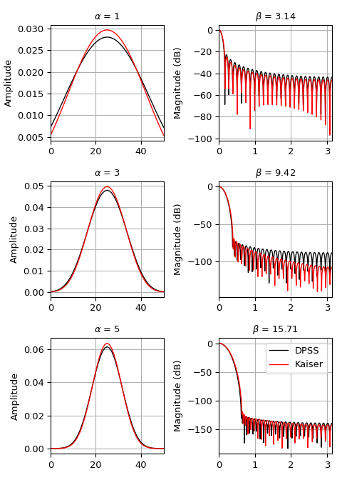
我們可以將此視窗與 kaiser 進行比較，後者被發明作為更容易計算的替代方案 [3]（範例改編自 此處）

>>> import numpy as np
>>> import matplotlib.pyplot as plt
>>> from scipy.signal import windows, freqz
>>> M = 51
>>> fig, axes = plt.subplots(3, 2, figsize=(5, 7))
>>> for ai, alpha in enumerate((1, 3, 5)):
...     win_dpss = windows.dpss(M, alpha)
...     beta = alpha*np.pi
...     win_kaiser = windows.kaiser(M, beta)
...     for win, c in ((win_dpss, 'k'), (win_kaiser, 'r')):
...         win /= win.sum()
...         axes[ai, 0].plot(win, color=c, lw=1.)
...         axes[ai, 0].set(xlim=[0, M-1], title=r'$\alpha$ = %s' % alpha,
...                         ylabel='Amplitude')
...         w, h = freqz(win)
...         axes[ai, 1].plot(w, 20 * np.log10(np.abs(h)), color=c, lw=1.)
...         axes[ai, 1].set(xlim=[0, np.pi],
...                         title=r'$\beta$ = %0.2f' % beta,
...                         ylabel='Magnitude (dB)')
>>> for ax in axes.ravel():
...     ax.grid(True)
>>> axes[2, 1].legend(['DPSS', 'Kaiser'])
>>> fig.tight_layout()
>>> plt.show()

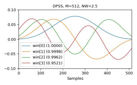
以下是前四個視窗的範例，以及它們的集中度比率

>>> M = 512
>>> NW = 2.5
>>> win, eigvals = windows.dpss(M, NW, 4, return_ratios=True)
>>> fig, ax = plt.subplots(1)
>>> ax.plot(win.T, linewidth=1.)
>>> ax.set(xlim=[0, M-1], ylim=[-0.1, 0.1], xlabel='Samples',
...        title='DPSS, M=%d, NW=%0.1f' % (M, NW))
>>> ax.legend(['win[%d] (%0.4f)' % (ii, ratio)
...            for ii, ratio in enumerate(eigvals)])
>>> fig.tight_layout()
>>> plt.show()

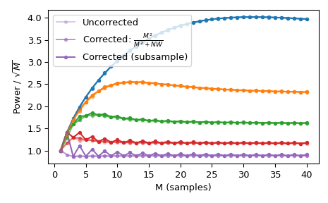
使用標準 \(l_{\infty}\) 範數會為偶數 M 產生兩個單位值，但僅為奇數 M 產生一個單位值。這會產生不均勻的視窗功率，可以通過近似校正 M**2/float(M**2+NW) 來抵消，可以通過使用 norm='approximate' 來選擇（這與 Kmax=None 時的 norm=None 相同，此處就是這種情況）。或者，可以使用較慢的 norm='subsample'，它使用頻域 (FFT) 中的子樣本位移來計算校正

>>> Ms = np.arange(1, 41)
>>> factors = (50, 20, 10, 5, 2.0001)
>>> energy = np.empty((3, len(Ms), len(factors)))
>>> for mi, M in enumerate(Ms):
...     for fi, factor in enumerate(factors):
...         NW = M / float(factor)
...         # Corrected using empirical approximation (default)
...         win = windows.dpss(M, NW)
...         energy[0, mi, fi] = np.sum(win ** 2) / np.sqrt(M)
...         # Corrected using subsample shifting
...         win = windows.dpss(M, NW, norm='subsample')
...         energy[1, mi, fi] = np.sum(win ** 2) / np.sqrt(M)
...         # Uncorrected (using l-infinity norm)
...         win /= win.max()
...         energy[2, mi, fi] = np.sum(win ** 2) / np.sqrt(M)
>>> fig, ax = plt.subplots(1)
>>> hs = ax.plot(Ms, energy[2], '-o', markersize=4,
...              markeredgecolor='none')
>>> leg = [hs[-1]]
>>> for hi, hh in enumerate(hs):
...     h1 = ax.plot(Ms, energy[0, :, hi], '-o', markersize=4,
...                  color=hh.get_color(), markeredgecolor='none',
...                  alpha=0.66)
...     h2 = ax.plot(Ms, energy[1, :, hi], '-o', markersize=4,
...                  color=hh.get_color(), markeredgecolor='none',
...                  alpha=0.33)
...     if hi == len(hs) - 1:
...         leg.insert(0, h1[0])
...         leg.insert(0, h2[0])
>>> ax.set(xlabel='M (samples)', ylabel=r'Power / $\sqrt{M}$')
>>> ax.legend(leg, ['Uncorrected', r'Corrected: $\frac{M^2}{M^2+NW}$',
...                 'Corrected (subsample)'])
>>> fig.tight_layout()

返回在新分頁中開啟