scipy.signal.windows.

chebwin

scipy.signal.windows.chebwin(M, at, sym=True)

傳回 Dolph-Chebyshev 視窗。

參數:

M整數

輸出視窗中的點數。如果為零，則傳回空陣列。當為負數時，會拋出例外。

at浮點數

衰減（分貝）。

sym布林值，選用

當 True（預設）時，產生對稱視窗，用於濾波器設計。當 False 時，產生週期性視窗，用於頻譜分析。

傳回值:

wndarray

視窗，最大值始終標準化為 1

註解

此視窗針對給定階數 M 和旁瓣等漣波衰減 at 優化最窄的主瓣寬度，使用 Chebyshev 多項式。它最初由 Dolph 開發，用於優化無線電天線陣列的方向性。

與大多數視窗不同，Dolph-Chebyshev 是根據其頻率響應定義的

\[W(k) = \frac {\cos\{M \cos^{-1}[\beta \cos(\frac{\pi k}{M})]\}} {\cosh[M \cosh^{-1}(\beta)]}\]

其中

\[\beta = \cosh \left [\frac{1}{M} \cosh^{-1}(10^\frac{A}{20}) \right ]\]

且 0 <= abs(k) <= M-1。A 是以分貝為單位的衰減 (at)。

時域視窗隨後使用 IFFT 生成，因此二次冪 M 生成速度最快，質數 M 生成速度最慢。

頻域中的等漣波條件在時域中產生脈衝，這些脈衝出現在視窗的末端。

參考文獻

[1]

C. Dolph, “A current distribution for broadside arrays which optimizes the relationship between beam width and side-lobe level”, Proceedings of the IEEE, Vol. 34, Issue 6

[2]

Peter Lynch, “The Dolph-Chebyshev Window: A Simple Optimal Filter”, American Meteorological Society (1997 年 4 月) http://mathsci.ucd.ie/~plynch/Publications/Dolph.pdf

[3]

F. J. Harris, “On the use of windows for harmonic analysis with the discrete Fourier transforms”, Proceedings of the IEEE, Vol. 66, No. 1, 1978 年 1 月

範例

在您的瀏覽器中試試看！

繪製視窗及其頻率響應圖

>>> import numpy as np
>>> from scipy import signal
>>> from scipy.fft import fft, fftshift
>>> import matplotlib.pyplot as plt

>>> window = signal.windows.chebwin(51, at=100)
>>> plt.plot(window)
>>> plt.title("Dolph-Chebyshev window (100 dB)")
>>> plt.ylabel("Amplitude")
>>> plt.xlabel("Sample")

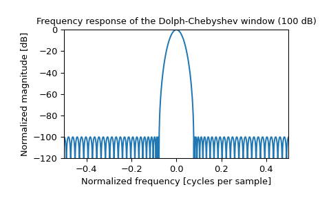
>>> plt.figure()
>>> A = fft(window, 2048) / (len(window)/2.0)
>>> freq = np.linspace(-0.5, 0.5, len(A))
>>> response = 20 * np.log10(np.abs(fftshift(A / abs(A).max())))
>>> plt.plot(freq, response)
>>> plt.axis([-0.5, 0.5, -120, 0])
>>> plt.title("Frequency response of the Dolph-Chebyshev window (100 dB)")
>>> plt.ylabel("Normalized magnitude [dB]")
>>> plt.xlabel("Normalized frequency [cycles per sample]")

返回在新分頁中開啟